
“Here’s the poly bag wiff our meals, Johnny. ‘S got two boxes innit, but no labels which is which.”
“I ordered the mutton pasty, Jennie, anna fish’n’chips for you.”
“You c’n have this box, Johnny. I’ll take the other one t’ my place to watch telly.”
…
<ring>
” ‘Ullo, Jennie? This is Johnny. The box over ‘ere ‘as the fish. You’ve got mine!”
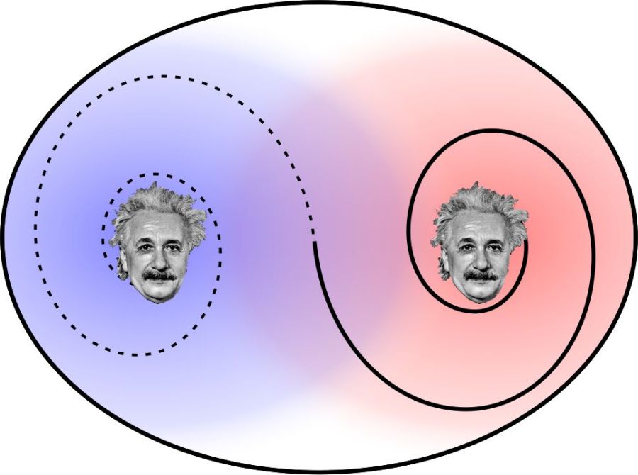
In a sense their supper order arrived in an entangled state. Our friends knew what was in both boxes together, but they didn’t know what was in either box separately. Kind of a Schrödinger’s Cat situation — they had to treat each box as 50% baked pasty and 50% fried codfish.
But as soon as Johnny opened one box, he knew what was in the other one even though it was somewhere else. Jennie could have been in the next room or the next town or the next planet — Johnnie would have known, instantly, which box had his meal no matter how far away that other box was.
By the way, Jennie was free to open her box on the way home but that’d make no difference to Johnnie — the box at his place would have stayed a mystery to him until either he opened it or he talked to her.
 Information transfer at infinite speed? Of course not, because neither hungry person knows what’s in either box until they open one or until they exchange information. Even Skype operates at light-speed (or slower).
But that’s not quite quantum entanglement, because there’s definite content (meat pie or batter-fried cod) in each box. In the quantum world, neither box holds something definite until at least one box is opened. At that point, ambiguity flees from both boxes in an act of global correlation.
There’s strong experimental evidence that entangled particles literally don’t know which way is up until one of them is observed. The paired particle instantaneously gets that message no matter how far away it is.
Niels Bohr’s Principle of Complementarity is involved here. He held that because it’s impossible to measure both wave and particle properties at the same time, a quantized entity acts as a wave globally and only becomes local when it stops somewhere.
Here’s how extreme the wave/particle global/local thing can get. Consider some nebula a million light-years away. A million years ago an electron wobbled in the nebular cloud, generating a spherical electromagnetic wave that expanded at light-speed throughout the Universe.

courtesy of NASA’s Hubble Space Telescope
Last night you got a glimpse of the nebula when that lightwave encountered a retinal cell in your eye. Instantly, all of the wave’s energy, acting as a photon, energized a single electron in your retina. That particular lightwave ceased to be active elsewhere in your eye or anywhere else on that million-light-year spherical shell.
Surely there was at least one other being, on Earth or somewhere else, that was looking towards the nebula when that wave passed by. They wouldn’t have seen your photon nor could you have seen any of theirs. Somehow your wave’s entire spherical shell, all 1012 square lightyears of it, instantaneously “knew” that your eye’s electron had extracted the wave’s energy.
But that directly contradicts a bedrock of Einstein’s Special Theory of Relativity. His fundamental assumption was that nothing (energy, matter or information) can go faster than the speed of light in vacuum. STR says it’s impossible for two distant points on that spherical wave to communicate in the way that quantum theory demands they must.
Want some irony? Back in 1906, Einstein himself “invented” the photon in one of his four “Annus mirabilis” papers. (The word “photon” didn’t come into use for another decade, but Einstein demonstrated the need for it.) Building on Planck’s work, Einstein showed that light must be emitted and absorbed as quantized packets of energy.
It must have taken a lot of courage to write that paper, because Maxwell’s wave theory of light had been firmly established for forty years prior and there’s a lot of evidence for it. Bottom line, though, is that Einstein is responsible for both sides of the wave/particle global/local puzzle that has bedeviled Physics for a century.
~~ Rich Olcott


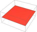

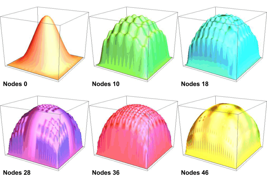
 Suppose you’re playing goalie in an inverse tennis game. There’s a player in each service box. Your job is to run the net line using your rackets to prevent either player from getting a ball into the opposing half-court. Basically, you want the ball’s locations to look like the single-node yellow shape up above. You’ll have to work hard to do that.



 I was only 10 years old but already had Space Fever thanks to Chesley Bonestell’s artwork in Collier’s and Life magazines. I eagerly joined the the movie theater ticket line to see George Pal’s Destination Moon. I loved the Woody Woodpecker cartoon (it’s 12 minutes into the


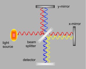 Their common experimental strategy sounds simple enough — compare two beams of light that had traveled along different paths


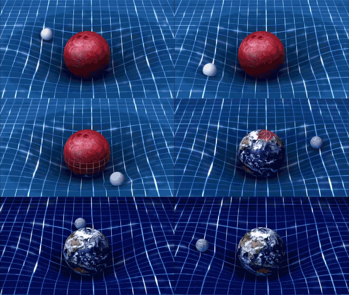
 Of all the wave varieties we’re familiar with, gravitational waves are most similar to (NOT identical with!!) sound waves. A sound wave consists of cycles of compression and expansion like you see in this graphic. Those dots could be particles in a gas (classic “sound waves”) or in a liquid (sonar) or neighboring atoms in a solid (a xylophone or marimba).
 Einstein noticed that implication of his Theory of General Relativity and in 1916 predicted that the path of starlight would be bent when it passed close to a heavy object like the Sun. The graphic shows a wave front passing through a static gravitational structure. Two points on the front each progress at one graph-paper increment per step. But the increments don’t match so the front as a whole changes direction. Sure enough, three years after Einstein’s prediction, Eddington observed just that effect while watching a total solar eclipse in the South Atlantic.
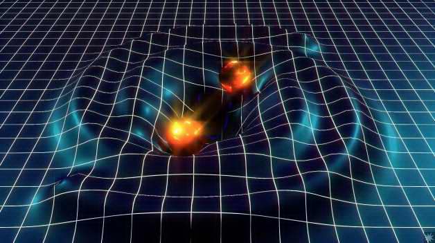
 We’re being dynamic here, so the simulation has to include the fact that changes in the mass configuration aren’t felt everywhere instantaneously. Einstein showed that space transmits gravitational waves at the speed of light, so I used a scaled “speed of light” in the calculation. You can see how each of the new features expands outward at a steady rate.
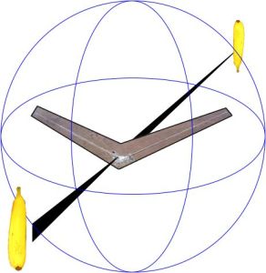 The second question is harder. The best the aLIGO team could do was point to a “banana-shaped region” (their words, not mine) that covers about 1% of the sky. The team marshaled a world-wide collaboration of observatories to scan that area (a huge search field by astronomical standards), looking for electromagnetic activities concurrent with the event they’d seen. Nobody saw any. That was part of the evidence that this collision involved two black holes. (If one or both of the objects had been something other than a black hole, the collision would have given off all kinds of photons.)
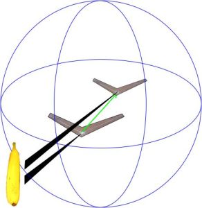 In contrast, a LIGO facility is (roughly speaking) omni-directional. When a LIGO installation senses a gravitational pulse, it could be coming down from the visible sky or up through the Earth from the other hemisphere — one signal doesn’t carry the “which way?” information. The diagram above shows that situation. (The “chevron” is an image of the LIGO in Hanford WA.) Models based on the signal from that pair of 4-km arms can narrow the source field to a “banana-shaped region,” but there’s still that 180o ambiguity.
 The great “if only” is that the VIRGO installation in Italy was not recording data when the Hanford WA and Livingston LA saw that September signal. With three recordings to reconcile, the aLIGO+VIRGO combination would have had enough information to slice that banana and localize the event precisely.

