Gin And The Art of Quantum Mechanics

“Fancy a card game, Johnny?”
“Sure, Jennie, deal me in.  Wot’re we playin’?”
“Gin rummy sound good?”


Great idea, and it fits right in with our current Entanglement theme.  The aspect of Entanglement that so bothered Einstein, “spooky action at a distance,” can be just as spooky close-up.  Check out this magic example — go ahead, it’s a fun trick to figure out.

Spooky, hey?  And it all has to do with cards being two-dimensional.  I know, as objects they’ve got three dimensions same as anyone (four, if you count time), but functionally they have only two dimensions — rank and suit.gin rummy hand

When you’re looking at a gin rummy hand you need to consider each dimension separately.  The queens in this hand form a set — three cards of the same rank.  So do the three nines.  In the suit dimension, the 4-5-6-7 run is a sequence of ranks all in the same suit.Gin rummy chart

A physicist might say that evaluating a gin rummy hand is a separable problem, because you can consider each dimension on its own. <Hmm … three queens, that’s a set, and three nines, another set.  The rest are hearts.  Hey, the hearts are in sequence, woo-hoo!> 

“Gin!”

If you chart the hand, the run and sets and their separated dimensions show up clearly even if you don’t know cards.

A standard strategy for working a complex physics problem is to look for a way to split one kind of motion out from what else is going on.  If the whole shebang is moving in the z-direction, you can address  the z-positions, z-velocities and z-forces as an isolated sub-problem and treat the x and y stuff separately.  Then, if everything is rotating in the xy plane you may be able to separate the angular motion from the in-and-out (radial) motion.

But sometimes things don’t break out so readily.  One nasty example would be several massive stars flying toward each other at odd angles as they all dive into a black hole.  Each of the stars is moving in the black hole’s weirdly twisted space, but it’s also tugged at by every other star.  An astrophysicist would call the problem non-separable and probably try simulating it in a computer instead of setting up a series of ugly calculus problems.Trick chart

The card trick video uses a little sleight-of-eye to fake a non-separable situation.  Here’s the chart, with green dots for the original set of cards and purple dots for the final hand after “I’ve removed the card you thought of.”  The kings are different, and so are the queens and jacks.  As you see, the reason the trick works is that the performer removed all the cards from the original hand.

The goal of the illusion is to confuse you by muddling ranks with suits.  What had been a king of diamonds in the first position became a king of spades, whereas the other king became a queen.  You were left with an entangled perception of each card’s two dimensions.

In quantum mechanics that kind of entanglement crops up any time you’ve got two particles with a common history.  It’s built into the math — the two particles evolve together and the model gives you no way to tell which is which.

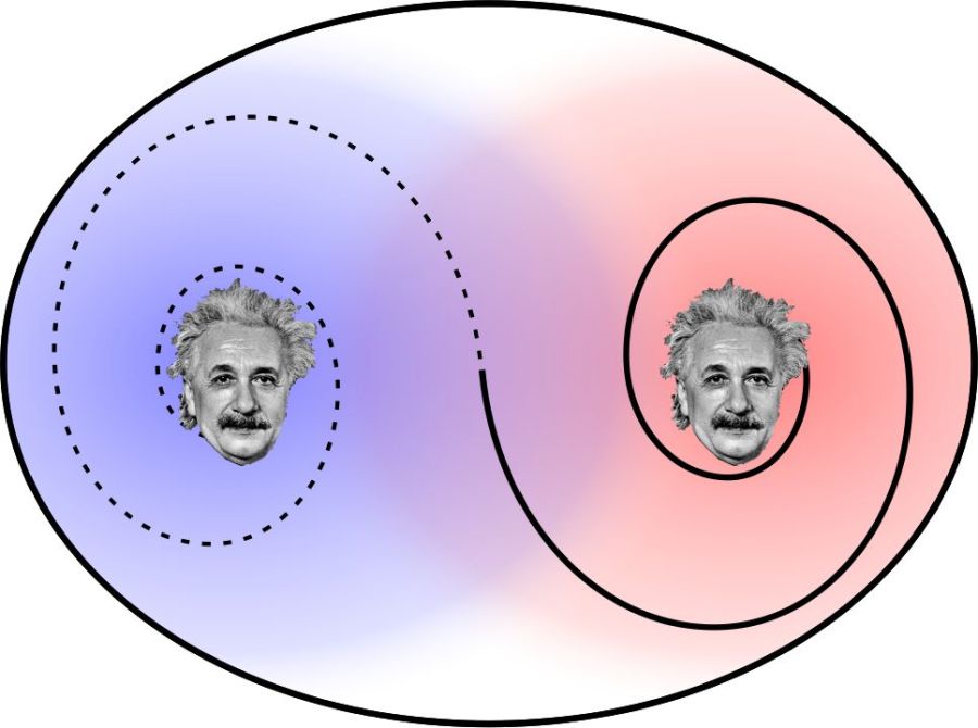
Suppose for instance that an electron pair has zero net spin  (spin direction is a dimension in QM like suit is a dimension in cards).  If the electron going to the left is spinning clockwise, the other one must be spinning counterclockwise.  Or the clockwise one may be the one going to the right — we just can’t tell from the math which is which until we test one of them.  The single test settles the matter for both.

Einstein didn’t like that ambiguity.  His intuition told him that QM’s statistics only summarize deeper happenings.  Bohr opposed that idea, holding that QM tells us all we can know about a system and that it’s nonsense to even speak of properties that cannot be measured.  Einstein called the deeper phenomena “elements of reality” though they’re currently referred to as “hidden variables.”  Bohr won the battle but maybe not the war — Einstein had such good intuition.

~~ Rich Olcott

Oh, what an entangled wave we weave

“Here’s the poly bag wiff our meals, Johnny.  ‘S got two boxes innit, but no labels which is which.”
“I ordered the mutton pasty, Jennie, anna fish’n’chips for you.”
“You c’n have this box, Johnny.  I’ll take the other one t’ my place to watch telly.”

<ring>
” ‘Ullo, Jennie?  This is Johnny.  The box over ‘ere ‘as the fish.  You’ve got mine!”


In a sense their supper order arrived in an entangled state.  Our friends knew what was in both boxes together, but they didn’t know what was in either box separately.  Kind of a Schrödinger’s Cat situation — they had to treat each box as 50% baked pasty and 50% fried codfish.

But as soon as Johnny opened one box, he knew what was in the other one even though it was somewhere else.  Jennie could have been in the next room or the next town or the next planet — Johnnie would have known, instantly, which box had his meal no matter how far away that other box was.

By the way, Jennie was free to open her box on the way home but that’d make no difference to Johnnie — the box at his place would have stayed a mystery to him until either he opened it or he talked to her.

Entangled 2Information transfer at infinite speed?  Of course not, because neither hungry person knows what’s in either box until they open one or until they exchange information.  Even Skype operates at light-speed (or slower).

But that’s not quite quantum entanglement, because there’s definite content (meat pie or batter-fried cod) in each box.  In the quantum world, neither box holds something definite until at least one box is opened.  At that point, ambiguity flees from both boxes in an act of global correlation.

There’s strong experimental evidence that entangled particles literally don’t know which way is up until one of them is observed.  The paired particle instantaneously gets that message no matter how far away it is.

Niels Bohr’s Principle of Complementarity is involved here.  He held that because it’s impossible to measure both wave and particle properties at the same time, a quantized entity acts as a wave globally and only becomes local when it stops somewhere.

Here’s how extreme the wave/particle global/local thing can get.  Consider some nebula a million light-years away.  A million years ago an electron wobbled in the nebular cloud, generating a spherical electromagnetic wave that expanded at light-speed throughout the Universe.

cats-eye nebula
The Cat’s Eye Nebula (NGC 6543)
courtesy of NASA’s Hubble Space Telescope

Last night you got a glimpse of the nebula when that lightwave encountered a retinal cell in your eye.  Instantly, all of the wave’s energy, acting as a photon, energized a single electron in your retina.  That particular lightwave ceased to be active elsewhere in your eye or anywhere else on that million-light-year spherical shell.

Surely there was at least one other being, on Earth or somewhere else, that was looking towards the nebula when that wave passed by.  They wouldn’t have seen your photon nor could you have seen any of theirs.  Somehow your wave’s entire spherical shell, all 1012 square lightyears of it, instantaneously “knew” that your eye’s electron had extracted the wave’s energy.

But that directly contradicts a bedrock of Einstein’s Special Theory of Relativity.  His fundamental assumption was that nothing (energy, matter or information) can go faster than the speed of light in vacuum.  STR says it’s impossible for two distant points on that spherical wave to communicate in the way that quantum theory demands they must.

Want some irony?  Back in 1906, Einstein himself “invented” the photon in one of his four “Annus mirabilis” papers.  (The word “photon” didn’t come into use for another decade, but Einstein demonstrated the need for it.)  Building on Planck’s work, Einstein showed that light must be emitted and absorbed as quantized packets of energy.

It must have taken a lot of courage to write that paper, because Maxwell’s wave theory of light had been firmly established for forty years prior and there’s a lot of evidence for it.  Bottom line, though, is that Einstein is responsible for both sides of the wave/particle global/local puzzle that has bedeviled Physics for a century.

~~ Rich Olcott

Think globally, act locally. Electrons do.

“Watcha, Johnnie, you sure ‘at particle’s inna box?”
“O’course ’tis, Jennie!  Why wouldn’t it be?”
“Me Mam sez particles can tunnel outta boxes ’cause they’re waves.”

“Can’t be both, Jessie.”


Double slit experiment
The double-slit experiment.
An electron beam travels from the source at left to a display screen. In between there’s a barrier with two narrow slits.

Maybe it can.

Nobel-winning (1965) physicist Richard Feynman said the double-slit experiment (diagrammed here) embodies the “central mystery” of Quantum Mechanics.

When the bottom slit is covered the display screen shows just what you’d expect — a bright area  opposite the top slit.

When both slits are open, the screen shows a banded pattern you see with waves.  Where a peak in a top-slit wave meets a peak in the bottom-slit wave, the screen shines brightly.  Where a peak meets a trough the two waves cancel and the screen is dark.  Overall there’s a series of stripes.  So electrons are waves, right?

But wait.  If we throttle the beam current way down, the display shows individual speckles where each electron hits.  So the electrons are particles, right?

Now for the spooky part.  If both slits are open to a throttled beam those singleton speckles don’t cluster behind the slits as you’d expect particles to do.  A speckle may appear anywhere on the screen, even in an apparently blocked-off region.  What’s more, when you send out many electrons one-by-one their individual hits cluster exactly where the bright stripes were when the beam was running full-on.

It’s as though each electron becomes a wave that goes through both slits, interferes with itself, and then goes back to being a particle!

By the way, this experiment isn’t a freak observation.  It’s been repeated with the same results many times, not just with electrons but also with light (photons), atoms, and even massive molecules like buckyballs (fullerene spheres that contain 60 carbon atoms).  In each case, the results indicate that the whatevers have a dual character — as a localized particle AND as a wave that reacts to the global environment.

Physicists have been arguing the “Which is it?” question ever since Louis-Victor-Pierre-Raymond, the 7th Duc de Broglie, raised it in his 1924 PhD Thesis (for which he received a Nobel Prize in 1929 — not bad for a beginner).  He showed that any moving “particle” comes along with a “wave” whose peak-to-peak wavelength is inversely proportional to the particle’s mass times its velocity.  The longer the wavelength, the less well you know where the thing is.

I just had to put numbers to de Broglie’s equation.  With Newton in mind, I measured one of the apples in my kitchen.  To scale everything, I assumed each object moved by one of its diameters per second.  (OK, I cheated for the electron — modern physics says it’s just a point, so I used a not-really-valid classical calculation to get something to work with.)

“Particle” Mass, kilograms Diameter, meters Wavelength, meters Wavelength, diameters
Apple 0.2 0.07 7.1×10⁻³³ 1.0×10⁻³¹
Buckyball 1.2×10⁻²⁴ 1.0×10⁻⁹ 0.083 8.3×10+7
Hydrogen atom 1.7×10⁻²⁷ 1.0×10⁻¹⁰ 600 6.0×10+12
Electron 9.1×10⁻³¹ 3.0×10⁻¹⁷ 3.7×10+12 1.2×10+29

That apple has a wave far smaller than any of its hydrogen atoms so I’ll have no trouble grabbing it for a bite.  Anything tinier than a small virus is spread way out unless it’s moving pretty fast, as in a beam apparatus.  For instance, an electron going at 1% of light-speed has a wavelength only a nanometer wide.

Different physicists have taken different positions on the “particle or wave?” question.  Duc de Broglie claimed that both exist — particles are real and they travel where their waves tell them to.  Bohr and Heisenberg went the opposite route, saying that the wave’s not real, it’s only a mathematical device for calculating relative probabilities for measuring this or that value.  Furthermore, the particle doesn’t exist as such until a measurement determines its location or momentum.  Einstein and Schrödinger liked particles.  Feynman and Dirac just threw up their hands and calculated.

Which brings us to the other kind of quantum spookiness — “entanglement.”  In fact, Einstein actually used the word spukhafte (German for “spooky”) in a discussion of the notion.  He really didn’t like it and for good reason — entanglement rudely collides with his own Theory of Relativity.  But that’s another story.

~~ Rich Olcott

Location, Location, Location

“Hoy, Johnny, still got that particle inna box?”
“Sure do, Jessie.”
“So where’s hit in there?”
“Me Pap says hit’s spread-out like but hit’s mostly inna middle.”
“Why’s hit spread then?”
“The more I taps the box, the wider hit spreads. Sommat to do wiff energy.”


PIB0
Newton would have answered Jessie’s question by saying, sort of, “Pick a point anywhere in the box.  The probability that the particle is at that point is equal to the probability that it’s at any other point.” PIB stack

Quantum physicists take a different approach. They start by saying, “We know there’s zero probability that the particle is anywhere outside of the box, so there must be zero probability that it’s exactly at any wall.”

Now for a trick that we’re actually quite used to.  When you listen to an orchestra, you can usually pick out the notes being played by a particular instrument.  Someone blessed/cursed with perfect pitch can tell when a note is just a leetle bit flat, say an A being played at 438 cycles instead of 440. You can create any sound by mixing together the right frequencies in the right proportion. That’s how an MP3 recorder does it.

QM solutions use that strategy the other way round. They calculate probabilities by adding together sets of symmetric elementary shapes, all of which are zero at certain places, like the box walls. For instance, on average Johnnie’s particle will be near the middle of his box, so we start a set with an orange mound of probability right there. That mound is like our base frequency — it has no nodes, no non-wall places where the probability is zero.

Then we add a first overtone, the one-node yellow shape that represents equal probability on either side of a plane of zero probability.

Two nodal planes at right angles give us the four-peaked green shape. Further steps up have more and more nodal planes (cyan then blue, and so on). The video shows the running total up to 46 nodes.

.PIB sum
As we add more nodes, the cumulative shape gets smoother and broader.  After a huge number of steps, the sum will look pretty much like Newton’s (except for right at the walls, of course).

So if the classical and QM boxes wind up looking the same, why go to all that trouble?  Because those nodes don’t come for free.

Inverse tennisSuppose you’re playing goalie in an inverse tennis game.  There’s a player in each service box.  Your job is to run the net line using your rackets to prevent either player from getting a ball into the opposing half-court.  Basically, you want the ball’s locations to look like the single-node yellow shape up above.  You’ll have to work hard to do that.

Now suppose they give you a second, crosswise net (the green shape).  You’re going to have to work twice as hard.  Now add a third net, and so on … each additional nodal plane is going to be harder (cost more energy) to keep empty.  Not a problem if you have an infinite amount of energy.

Enter Planck and Einstein.  They showed there’s a limit for small systems like atoms and molecules.  Electrons dash about in atom- or molecule-shaped boxes, but the principle is the same.  The total probability distribution is still the sum of bounded elementary shapes.  However, you can’t use an infinite number of them.  Rather, you start with the cheapest shapes (the fewest nodes) and build upward.

Tally two electrons for each shape you use.  Why two?  Because that’s the rule, no arguments.

It’s important to realize that QM does NOT say that two specific electrons occupy one shape.  All the charge is spread out over all the shapes — we’re just keeping count.

When you run out of electrons the accumulated model shows everything we can know about the electronic configuration.  You won’t know where any particular electron is, but you’ll know where some electron spends some time.  For a chemist that’s the important thing — the peaks and nodes, the centers of negative and positive charge, are the most likely regions for chemical reactions to happen.

Johnnie’s energetic taps make his particle boldly go where no particle has gone before.

~~ Rich Olcott

Particles and Poetry

“Hoy, Johnny, wotcher got inna box?”
“Hit’s a particle, Jessie.”
“Ooo, lovely for you.  Umm… wot’s a particle then?”
“Me Pap says hit’s sommat you calc’late about wiffout knowin’ wot ’tis.”


Pap’s right.  Newton was a particle guy all the way (he was a strong supporter of the idea that light is composed of particles).  One of his most important insights was that he could simplify gravitational calculations if he replaced an object with an equally massive “particle” located at the object’s center of mass.  Could be a planet, or a moon, or that apple — he could treat each of them as a “particle.”  That worked fine for his purposes, because the distances between his object centers were vastly larger than the object sizes.

Fleas
“Great fleas have little fleas upon their backs to bite ’em / And little fleas have lesser fleas and so on infinitum.” ~~ Augustus De Morgan

It took Roche to work out what happens when the distances get small.  Gravitational forces break the original “particles” into littler particles.  And when two of the little ones approach closely enough they break up, and then those break up…  You get the idea.  Take the process far enough and you get Saturn’s Rings, for instance.

But the analysis can keep going.  Consider one “particle” in Saturn’s A-ring.  It’s probably about 3″ across, made of ice, and contains something like 1024 particles that happen to be molecules of H2O.  Each molecule contains 3 nuclei (2 protons and one oxygen nucleus) and 10 electrons, all 13 of which merit “particle” status if you’re calculating molecules.  They’re all held together by a blizzard of photons carrying the electromagnetic forces between them.  The oxygen nucleus contains 16 nuclear particles, each of which contains 3 quarks.  The quark structures would fly apart except for a host of gluons that pass back and forth transmitting the nuclear strong force.  Hooboy, do we got particles.

“Particle” is a slippery word.  For Newton’s purposes, if an object is small relative to its distance from other objects, that was all he needed to know to treat it as a particle.

One dictionary specifies “a small localized object which has identifiable physical or chemical properties such as volume or mass.”  However, there are theoretical grounds to believe that the classic “particle of light,” the photon, has neither mass nor volume.  Physicists have had long arguments trying to devise a good working definition.  Nobelist (1999) Gerard ‘t Hooft ended one such discussion by saying, “A particle is fundamental when it’s useful to think of it as fundamental.”

It may seem a little strange for a physicist to argue for imprecision.  In fact, ‘t Hooft was arguing for a broad, even poetic but still precise understanding of the word.

Poets use metaphor to help us understand the world.  Part of their art is to pack as much meaning as they can into the minimum number of words.  In the same way, scientists use mathematics to pack observed relationships into a simile called an equation  — a brief bit of math may connect and illuminate many disparate phenomena.

Think of physics as metaphor, with numbers.

Newton’s Law of Gravity works for for galaxies roving through a cluster and for basketball-sized satellites orbiting Earth and for stars circling a black hole (if they don’t get too close).  Maxwell’s Equations, just 30 symbols including parentheses and equal signs, give the speed of light and describe the operation of electric motors.  The particle physicists’ Standard Model makes predictions that match experimental results to more than a dozen decimal places.

Good equations are so successful that Nobelist (1963) Eugene Wigner wrote an influential paper entitled The Unreasonable Effectiveness of Mathematics in the Natural Sciences.

We sometimes get into trouble by confusing metaphor with reality.  Poetic metaphors can be carried too far — Hamlet’s lungs were not in fact filling with water from his “sea of troubles.”

Mathematical models can also be carried too far.  Popular (and practitioner) discussion of quantum mechanics is rife with over-extended metaphors.  QM calculations yield only statistical results — an average position, say, plus or minus so much.  It’s an average, but of what?  The “many worlds” hypothesis is an unnecessarily long jump.  There are simpler, less extravagant ways to account for statistical uncertainty. les Etats Unis

~~ Rich Olcott

Perturbed? You’re not the only one

Dolls
Successive approximations
to a real girl, but still not there

It started with the Babylonians.  The Greeks abhorred the notion.  The Egyptians and Romans couldn’t have gotten along without it. Only 1600 years later did Newton gave final polishing to … The Method of Successive Approximations.

Stay with me, we’ll get to The Chicken soon.

Suppose for some weird reason you wanted to know the square root of 2701.  Any Babylonian could see immediately that 2701 is a bit less than 3600 = 602, so as a first approximation they’d guess ½(60 + (2701/60)) = 52.5.  They’d do the multiplication to check: 52.5×52.5 = 2756.25.

Well, 52.5 is closer than 60 but not close enough.  So they’d plug that number into the same formula to get the next successive approximation: ½(52.5 + 2701/52.5) = 51.97.  Check it: 51.97×51.97 = 2700.88.  That was probably good enough for government work in Babylonia, but if the boss wanted an even better estimate they could go around the loop again.

Scientists and engineers tackle a complex problem piecewise.  Start by looking for a simple problem you know how to solve. Adjust that solution little by little to account for the ways in which the real system differs from the simple case.  Successive Approximation is only one of many adjustment strategies invented over the centuries.

The most widely-used technique is called Perturbation Theory (which has nothing to do with the ways kids find to get on their parents’ nerves).  The strategy is to find some single parameter, maybe a ratio of two masses or the relative strength of a particle-particle interaction.  For a realistic solution, it’s important that the parameter’s value be small compared to other quantities in the problem.

Simplify the original problem by keeping that parameter in the equations but assume that it’s zero.  When you’ve found a solution to that problem, you “perturb” the solution — you see what happens to the model when you allow the parameter to be non-zero.

There’s an old story, famous among physicists and engineers, about an association of farmers who wanted to design an optimum chicken-raising operation.  Maybe with an optimal chicken house they could heat the place with the birds’ own body heat, things like that.  They called in an engineering consultant.  He looked around some running farms, took lots of measurements, and went away to compute.  A couple of weeks later he came back, with slides.  (I told you it’s an old story.)  He started to walk the group though his logic, but he lost them when he opened his pitch with, “Assume a spherical chicken…”

Fat chick bank
Henrietta
Fat Chicken Bank by Becky Zee

Now, he may actually have been on the right track.  It’s a known fact that many biological processes (digestion, metabolism, drug dosage, etc.) depend on an organism’s surface area.  A chicken’s surface area could be key to calculating her heat production.  But chickens (for example, our charming Henrietta) have a complicated shape with a poorly-defined surface area.  The engineer’s approximation strategy must have been to estimate each bird as a sphere with a tweakable perturbation parameter reflecting how spherical they aren’t.

Then, of course, he’d have to apply a second adjustment for feathers, but I digress.

Now here’s the thing.  In quantum mechanics there’s only a half-dozen generic systems with exact solutions qualifying them to be “simple” Perturbation Theory starters.  Johnny’s beloved Particle In A Box (coming next week) is one of them.  The others all depend in similar logic — the particle (there’s always only one of them) is confined to a region which contains places where the particle’s not allowed to be. (There’s one exception: the Free Particle has no boundaries and therefore is evenly smeared across the Universe.)

Virtually all other quantum-based results — multi-electron atoms, molecular structures, Feynman diagrams for sub-atomic physics, string theories, whatever — depend on Perturbation Theory.  (The exceptions are topology and group-theory techniques that generally attempt to produce qualitative rather quantitative predictions.)  They need those tweakable parameters.

In quantum-chemical calculations the perturbation parameters are generally reasonably small or at least controllable.  That’s not true for many of the other areas.  This issue is especially problematic for string theory.  In many of its proposed problem solutions no-one knows whether a first-, second- or higher-level approximation even exists, much less whether it would produce reasonable predictions.

I find that perturbing.

~~ Rich Olcott

The Universe and Werner H.

Heisenberg’s Area ( about 10-34 Joule-second) is small, one ten-millionth of the explosive action in a single molecule of TNT.  OK, that’s maybe important for sub-atomic physics, but it’s way too small to have any implications for anything bigger, right?  Well, it could be responsible for shaping our Universe.

Quick recap: The Heisenberg Uncertainty Principle (HUP) says that certain quantities (for instance, position and momentum) are linked in a remarkable way.  We can’t measure either of them perfectly accurately, but we can make repeated more-or-less sloppy measurements that give us average values.  The linkage is in that sloppiness.  Each repeated measurement lands somewhere in a range of values around the average.  HUP says that even with very careful measurement the product of those two spans must be greater than Heisenberg’s Area.

So now let’s head out to empty space, shall we?  I mean, really empty space, out there between the galaxies, where there’s only about one hydrogen atom per cubic meter.

Here’s a good cubic meter … sure enough, it’s got exactly one hydrogen atom in it.

g25For practice using Heisenberg’s Area, what can we say about the atom? (If you’re checking my math it’ll help to know that the Area, h/4π, can also be expressed as 0.5×10⁻³⁴ kg m2/s; the mass of one hydrogen atom is 1.7×10⁻²⁷ kg; and the speed of light is 3×10⁸ m/s.)  On average the atom’s position is at the cube’s center.  Its position range is one meter wide.  Whatever the atom’s average momentum might be, our measurements would be somewhere within a momentum range of (h/4π kg m2/s) / (1 m) = 0.5×10⁻³⁴ kg m/s. A moving particle’s momentum is its mass times its velocity, so the velocity range is (0.5×10⁻³⁴ kg m/s) / (1.7×10⁻²⁷ kg) = 0.3×10⁻⁷ m/s.

With really good tools we could determine the atom’s velocity within plus or minus 0.000 000 03 m/s.  Pretty good.

Now zoom in.  Dial that one-meter cube down a billion-fold to a nanometer (10-9 meters, which is still about ten times the atom’s width).  Yeah, the atom’s still in the box, but now its velocity range is 300 m/s.  The atom could be just hanging out at the center, or it could zoom out of the cube a microsecond after we looked — we just can’t tell which.

All of which illuminates the contrast between physics Newton-style and the physics that has bloomed since Einstein’s 1905 “miracle year.”  If Newton were in charge of the Universe, Heisenberg’s Area would be zero.  We could determine that atom’s position and momentum with complete accuracy.  In fact in principle we could accurately determine everything’s position and momentum and then calculate where everything would be at any time in the future.  But he isn’t and it’s not and we can’t.

Theorists and experimenters use the word “measurement” in different ways. A measurement done by a theoretician is generally based on fundamental constants and an Values
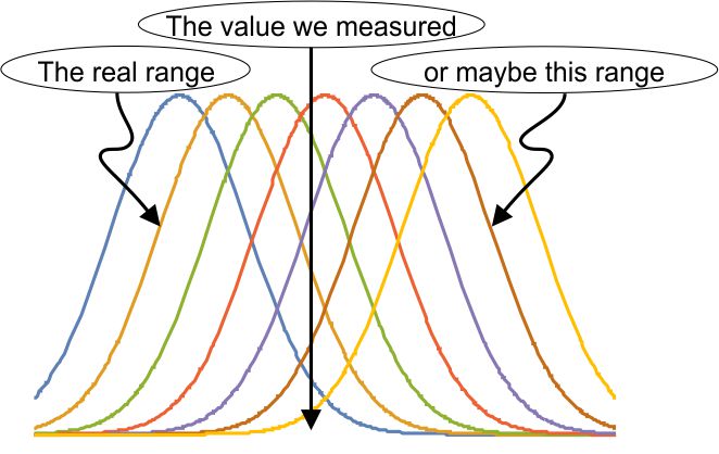
elaborate mathematical structure. If the measurement is a quantum mechanical result, part of that structure is our familiar bell-shaped curve.  It’s an explicit recognition that way down in the world of the very small, we can’t know what’s really going on.  Most calculations have to be statistical, predicting an average and an expected range about that average. That prediction may or may not pan out, depending on what the experimentalists find.

By contrast, when experimenters measure something, even as an average of multiple tests, it’s an estimate of the real distribution.  The research group (usually it’s a group these days) reports a distribution that they claim overlaps well with a real one out there in the Universe.  Then another group dives in to prove they or the theoreticians or both are wrong.  That’s how Science works.

You are hereSo there could be a collection of bell-curves gathered about the experimental result. Remember those extra dimensions we discussed earlier?  One theory that’s been floated is that along those extra dimensions the fundamental constants like h might take on different values.  Maybe further along “Dimension W” the value of h is bigger than it is in our Universe, and quantum effects are even more important than they are here.

Now how can we test that?

BTW, Heisenberg will be 114 on Dec 5.  Alles Gute zum Geburtstag, Werner!

~~ Rich Olcott

Heisenberg’s Area

Unlike politicians, scientists want to know what they’re talking about when they use a technical word like  “Uncertainty.”  When Heisenberg laid out his Uncertainty Principle, he wasn’t talking about doubt.  He was talking about how closely experimental results can cluster together, and he was putting that in numbers.

ArrowsThink of Robin Hood competing for the Golden Arrow.  For the showmanship of the thing, Robin wasn’t just trying to hit the target, he wanted his arrow to split the Sheriff’s.  If the Sheriff’s shot was in the second ring (moderate accuracy, from the target’s point of view), then Robin’s had to hit exactly the same off-center location (still moderate accuracy but great precision).  The Heisenberg Uncertainty Principle (HUP) is all about precision (a.k.a, range of variation).

We’ve all encountered exams that were graded “on the curve.”  But what curve is that?  I can say from personal experience that it’s extraordinarily difficult to create an exam where  the average grade is 75.  I want to give everyone the chance to show what they’ve learned.  Each student probably learned only part of what’s in the unit, but I won’t know which part until after the exam is graded.  The only way to be fair is to ask about everything in the unit.  Students complained that my tests were really hard because to get 100 they had to know it all.

Translating test scores to grades for a small class was straightforward.  I would plot how many papers got between 95 and 100, how many got 90-95, etc, and look at the graph.  Nearly always it looked like the top example.  TestsThere’s a few people who clearly have the material down pat; they clearly earned an “A.”  Then there’s a second group who didn’t do as well as the A’s but did significantly better than the rest of the class — they earned a “B.”  As the other end there’s a (hopefully small) group of students who are floundering.  Long-term I tried to give them extra help but short-term I had no choice but to give them an “F.”

With a large class those distinctions get blurred and all I saw (usually) was a single broad range of scores, the well-known “bell-shaped curve.”  If the test was easy the bell was centered around a high score.  If the test was hard that center was much lower.  What’s interesting, though, is that the width of that bell for a given class stayed pretty much the same.  The curve’s width is described by a number called the standard deviation (SD), proportional to the width at half-height.  If a student asked, “What’s my score?” I could look at the curve for that exam and say there’s a 66% chance that the score was within one SD of the average, and a 95% chance that it was within two SD’s.

The same bell-shape also shows up in research situations where a scientist wants to measure some real-world number, be it an asteroid’s weight or elephant gestation time.  He can’t know the true value, so instead he makes many replicate measurements or pays close attention to many pregnant elephants.  He summarizes his results by reporting the average of all the measurements and also the SD calculated from those measurements.  Just as for the exams, there’s a 95% chance that the true value is within two SD’s of the average.  The scientist would say that the SD represents the uncertainty of the measured average.

Which is what Heisenberg’s inequality is about.  Heisenberg area 1He wrote that the product of two paired uncertainties (like position and momentum) must be larger than that teeny “quantum of action,” h.  There’s a trade-off.  We can refine our measurement of one variable but we’ll lose precision on the other.  If we plot results for one member of the pair against results for the other, there’s no linkage between their average values.  However, there will be a rectangle in the middle representing the combined uncertainty.

Heisenberg tells us that the minimum area of that rectangle is a constant.

It’s a very small rectangle, area = h/4π = 0.5×10⁻³⁴ Joule-sec, but it’s significant on the scale of atoms — and maybe on the scale of the Universe (see next week).

~~ Rich Olcott

Heisenberg’s trade-offs

KiteA kite floating on the breeze.  Optimal work-life balance.  Smoothly functioning free markets.  The Heisenberg Uncertainty Principle.  Why would an alien from another planet recognize the last one but maybe not the others?

The kite is a physical object, intentionally built by humans to human scale.  The next two are idealized theoretical constructs, goals to be approached but rarely achieved.  The Heisenberg Uncertainty Principle (HUP) is fundamental to how the Universe works.

The first three are each in a dynamic equilibrium that is constantly buffeted by competing forces.  The HUP comes straight out of the deep math for where those forces come from.  Kites and work stress and markets may be peculiar to Earth, but the HUP is in play on every planet and star.

In the last post we saw that thanks to the HUP we can precisely identify an oboe’s pitch if it plays forever.  We can know precisely when a pitchless cymbal crashed.  But it’s mathematically impossible to get both exact pitch and exact time for the same sound.  Thank goodness, we can have imprecise knowledge of both quantities and actually play some music.

We determine a pitch (cycles per second) by counting sound waves passing during a given duration — and that limits our knowledge.  We can’t know that a wave has passed unless we see at least two peaks.  Our observation period must be at least long enough to see two peaks.  To put it the other way, the pitch must be high enough to give us at least two peaks during the time we’re watching.  This isn’t quantum mechanics, it’s just arithmetic, but it’s basic to physics.

Mathematically the HUP is as simple as Einstein’s E=mc2 equation, except the HUP is an inequality:

[A-uncertainty] x [B-uncertainty] ≥ h / 4π

where A and B are two paired quantities like pitch and duration.

TNT(That h is Planck’s constant, “the quantum of action,” 6.6×10⁻³⁴ joule-sec.  That’s a very small number indeed but it shows up everywhere in quantum physics.  To put h in scale, one gram of TNT packs 4184 joules of explosive energy.  TNT has a detonation velocity of 6900 meters/sec and density of 1.60 gram/cm3, so we can figure a 1-gram cube of the stuff would burn for 1.2 microseconds and generate a total action of about 5×10⁻³ joule-sec.  Divide that by Avagadro’s number to get that one molecule of TNT is good for 10-26 joule-sec.  That’s about 10 million times h.  So, yeah, h is small.)

Back to the HUP inequality.  A and B are our paired quantities.  The standard examples that everyone’s heard of are position and momentum, as in the old physicist joke, “I haven’t a clue where I’m going, but I know how fast I’m getting there.”  For things that are tied to a central attractor like an atomic nucleus, A and B would be angular position and angular momentum.  If you’re into solid-state physics you may have run into another example — the number of electrons in a superconducting current is paired with a metric that reflects the degree of order in the conducting medium.  One more pair is energy and time, but that’s a story for another week.

Balance 1But what’s in the HUP inequality isn’t A and B, but rather our uncertainty about each.  A billiard ball might be on the lip of the near cup or it can be all the way across the table — HUP won’t care.  What’s important to HUP is whether the ball is here plus/minus one inch, or here plus/minus a millionth of an inch.  Similarly, HUP doesn’t care how fast the ball is going, but it does care whether the speed is plus/minus one inch per second or plus/minus one millionth of an inch per second.  HUP tells us that we can know one of the pair precisely and the other not at all, or that we can know both imprecisely.  Furthermore, even the imprecision has a limit.

We can’t simultaneously know both A and B more precisely than that little teeny h, but some physicists believe h may have been big enough to launch our Universe.

Next week — HUP, two, three, four

~~ Rich Olcott

Don’t blame Heisenberg

There was the time I discovered that a chemical compound I’d made is destroyed by the light of the spectrometer I was using to study it. The NYT just ran an article about how biologists have a new-tech problem studying animals in the field because a camera drone can scare the critters away (or provoke an attack).  A teacher can’t shut down an ongoing bullying campaign because student chatter stops when they see him coming.  What’s the common thread in these situations?

You probably thought “Heisenberg,” but please don’t dis the poor guy for them.  You may have seen the for-real Heisenberg Uncertainty Principle in action, but only if you’re a physicist or a music-reading percussionist.  Rather, the incidents in the first paragraph are all examples of the Observer Effect, which is completely separate from the work of Werner H.

The confusion arises because the Observer Effect is often used in classroom explanations of the Heisenberg Uncertainty Principle (the HUP).  The Observer Effect could well apply pretty much anywhere there’s an observer and an observee (see photo), which is why research psychologists and police interrogators use one-way mirrors.

By contrast, the HUP is in play in only a few circumstances, chiefly audio and physics labs.  The key is that word uncertainty, because the HUP is all about the limits of our knowledge.  It says that there are certain pairs of quantities where we must trade off knowledge of one against knowledge of the other.  The more precisely we know the value of one, the more uncertain we are about the other one’s value.

drum notesLet’s start with sound.  Did you know that sheet music for a drummer doesn’t really use a “proper” staff with keys and all?  Oh, sure, they use a staff, sort of, but the “notes” indicate strokes rather than tones.  Here’s one variant of many notations out there.

Suppose an oboist plays a tone for you, that nice, long “A” that the orchestra tunes to.  (It’s generally the oboe playing that note, by the way, for two reasons.  First, the oboe uses very little air to produce its sound, so the oboist can hold that note much longer than a flautist or trumpeter could.  More important, though, is that the oboe simply isn’t adjustable — everyone else perforce has to re-tune to match up.)  The primary component of that “A” sound should be a wave of 440 cycles per second.

Now suppose the oboist plays that “A” in shorter and shorter bursts — half-note, quarter-note, etc., down to where all that comes out is a blip.  His fingering and embouchure don’t change, so he’s still playing an “A.” However, when the emitted sound wave is very short we can no longer identify the pitch because there aren’t enough cycles there.  We need at least 2 cycles in a known time period to be able to say how many cycles per second the tone has.

Now the oboist switches up an octave (880 cycles per second) with the same burst length.  That gives us twice as many cycles in the blip and we can identify the new pitch.  However, if he cuts the note’s length in half once more, then again we don’t have enough cycles to count.  The shorter the note, the more precisely we know when it sounded, but the less precisely we know what note it was.

A cymbal crash is basically the limiting case.  It has no distinct pitch (or the physicist would say it has a huge number of pitches that all die away after a few cycles).  Rather than tell the percussionist to play an unidentifiably short note, the composer says, “T’heck with it!” and writes an “X” somewhere on the staff.

And vice-versa — at the start of the oboist’s note the sound contained an mixture of other frequencies.  The interlopers eventually died out as the note proceeded.  There will be another mixing when the oboist runs out of breath.  We can only have a really pure tone if the note never starts and never ends — the poor oboist plays that one note forever.

Thank to Heisenberg, we can be confident that even Bach’s well-tempered clavier was imprecise.

Next week — more fun with Heisenberg.

~~ Rich Olcott