Shapes And Numbers

I’m nursing my usual mug of eye‑opener in Cal’s Coffee Shop when astronomer Cathleen and chemist Susan chatter in and head for my table. Susan fires the first volley.

“Sy, those spherical harmonics you’ve posted don’t look anything like the atomic orbitals in my Chem text. Shouldn’t they?”
 ”How do you add and multiply shapes together?”
  ”What does the result even mean?”
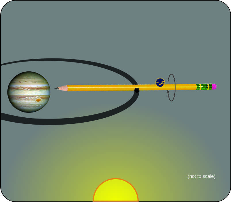
   ”And what was that about solar seismology?”

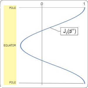
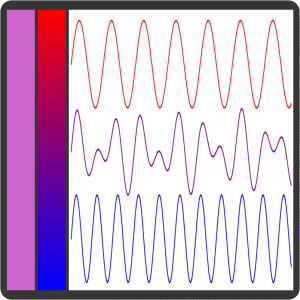
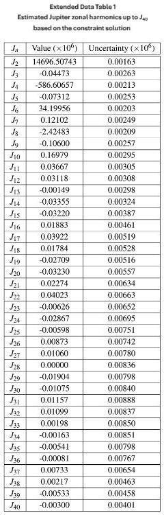
“Whoa, have you guys taken interrogation lessons from Mr Feder? One at a time, please. Let’s start with the basics.” <sketching on a paper napkin> “For example, the J2 zonal harmonic depends only on the latitude, not on the longitude or the distance from the center, so whatever it does encircles the axis. Starting at the north pole and swinging down to the south pole, the blue line shows how J2 varies from 1.0 down to some negative decimal. At any latitude, whatever else is going on will be multiplied by the local value of J2.”

“The maximum is 1.0, huh? Something multiplied by a number less than 1 becomes even smaller. But what happens where J2 is zero? Or goes negative?”

“Wherever Jn‘s zero you’re multiplying by zero which makes that location a node. Furthermore, the zero extends along its latitude all around the sphere so the node’s a ring. J2‘s negative value range does just what you’d expect it to — multiply by the magnitude but flip the product’s sign. No real problem with that, but can you see the problem in drawing a polar graph of it?”

“Sure. The radius in a polar graph starts from zero at the center. A negative radius wouldn’t make sense mixed in with positives in the opposite direction.”

“Well it can, Cathleen, but you need to label it properly, make the negative region a different color or something. There are other ways to handle the problem. The most common is to square everything.” <another paper napkin> “That makes all the values positive.”

“But squaring a magnitude less than 1 makes it an even smaller multiplier.”

“That does distort the shapes a bit but it has absolutely no effect on where the nodes are. ’Nothin’ times nothin’ is nothin’,’ like the song says. Many of the Chem text orbital illustrations I’ve seen emphasize the peaks and nodes. That’s exactly what you’d get from a square‑everything approach. Makes sense in a quantum context, because the squared functions model electron charge distributions.”

“Thanks for the nod, Sy. We chemists care about charge peaks and nodes around atoms because they control molecular structures. Chemical bonds and reactions tend to localize near those places.”

“I aim for fairness, Susan. There is another way to handle a negative radius but it needs more context to look reasonable. Meanwhile, we’ve established that at any given latitude each Jn is just a number so let’s look at longitudes.” <a third paper napkin> “Here’s the first two sectorial harmonics plotted out in linear coordinates.”

“Looks familiar.”

“Mm‑hm. Similar principles, except that we’re looking at a full circle and the value at 360° must match the value at 0°. That’s why Cm always has an even node count — with an odd number you’d have -1 facing +1 and that’s not stable. In polar coordinates,” <the fourth paper napkin> “it’s like you’re looking down at the north pole. C0 says ‘no directional dependence,’ but C1 plays favorites. By the way, see how C1‘s negative radii in the 90°‑270° range flip direction to cover up the positives?”

“Ah, I see where you’re going, Sy. Each of these harmonics has a numeric value at each angle around the center. You’re going to tell us that we can multiply the shapes by multiplying their values point by point, one for each latitude for a J and each longitude for a C.”

“You’re way ahead of me as usual, Cathleen. You with us, Susan?”

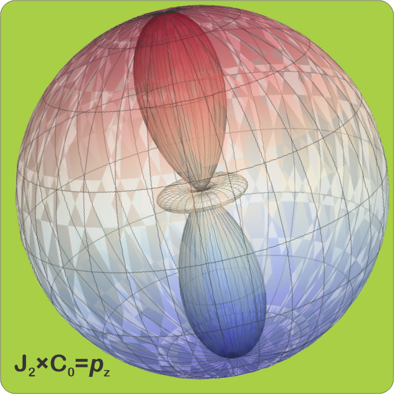
“Oh, yes. In my head I multiplied your J2 by C0 and got a pz orbital.”

“I’m impressed.”
 ”Me, too.”

“Oh, I didn’t do it numerically. I just followed the nodes. J2 has two latitude nodes, C0 has no longitude nodes. There it is, easy‑peasy.”

~~ Rich Olcott

Sectorial Setbacks

<chirp, chirp> “Moire here.”

“Moire, you were holding out on me. Eddie’s, fifteen minutes.”

“Not so fast, Walt. That wasn’t me holding out, that was you leaving too soon. From now on you’re paying quite a bit more. And it’ll be thirty minutes.”

“So we’re negotiating, hmm?”

“That’s about the size of it. You still interested?”

“My people are, they sent me back here. Oh well. Thirty minutes.”


Thirty-three minutes later I walk into Eddie’s. Walt’s already gotten a table. He beckons, points to the freshly‑served pizza, raises an eyebrow.

“Apology accepted. What made your people unhappy?”

“You told me flat‑out that the Sun’s gravity couldn’t affect those zonal harmonics. Do you have anything to back that up?”

“Symmetry. Zonal harmonics and latitude are about north‑south. Each Jn is a pole‑to‑pole variation pattern. The only way solar gravity can tilt Jupiter’s north‑south axis is to exert torque along the zonal harmonics. Jupiter’s equator is within 3° of edge‑on to the Sun.” <showing an image on Old Reliable’s screen> “Here’s what the Sun sees looking at J10, for instance. Solar pull on any northern zone segment, say, would be counteracted by an equal pull on the corresponding southern segment of the same zone. No net torque, no tilt. J0‘s the only exception. It’s simply a sphere that doesn’t vary across the whole planet. The Sun’s pull along J0‘s arc can’t tilt Jupiter.”

“Okay, so the zonal picture’s too simple. Just one set of waves, running up and down the planet—”

“No, not running. One way to characterize a wave is by how its components change with time. You’re thinking like ocean waves that move from place to place as time goes by. There’s also standing waves like on a guitar string, where individual points move but the peaks and valleys don’t. There’s time‑only waves like how the day length here changes through the year. And there’s static waves where time’s not even in the equation. Jupiter’s stripes don’t move, they’re peaks and valleys in a static wave pattern. By definition, the zonal harmonic system is static like that. But you’re right, it’s only part of the picture.”

“Give me the part the Sun’s gravitational field does play with.”

“That’d be two parts — sectorial and radial harmonics. Sectorial is zonal’s perpendicular twin. Zonal wave patterns show variation along the polar axis; sectorial wave patterns Cm vary around it. I’m keeping it non‑technical for you but Cm‘s actually cos(m*x) where x is the longitude.”

“Just don’t let it go any farther.”

“I’ll try not to. My point is that each sector pattern can be labeled with a positive integer just like we did with the zones.”

“If the Jn arcs aren’t affected by solar gravity, why would I care about these Cms?”

“You wouldn’t, except for the fact that mass distribution across Jupiter’s sectors is probably lumpy. We know the Great Red Spot holds its position in the southern hemisphere and the planet’s magnetic field points way off to the side. Maybe those features mark off‑center mass deficits and concentrations. Suppose a particular sectorial wave’s peak sits directly over a mass lump or hole. Everything under that harmonic’s influence is tugged back and forth by solar gravity each time the wave traverses the day side. Juno in its N‑S path just isn’t an efficient sensor for those tugs. Good sectorial sensing would require an orbiter on an E‑W path, preferably right over the equator.  Any orbital wobbles we’d see could be fed into a sectorial gravity map. Cross that with the zonal map and we’d be able to locate underlying mass variations by latitude and longitude.”

“Not a good idea. Gravity’s not the only field in play. You’ve just mentioned Jupiter’s magnetic field. I’ve read it’s stronger than any other planet’s. If your E‑W orbiter’s built with even a small amount of iron, you’d have a hard time deciding which field was responsible for any observed irregularities.”

“Good point. The idea’s even worse than you think, though. Jupiter’s sulfur‑coated moon—”

“Io. Yes, your induction‑heating idea might even be real. What about it?”

“I haven’t written yet about the high‑voltage Io‑to‑Jupiter bridge made of sulfur, oxygen and hydrogen ions. Jupiter’s magnetism plays a complicated game with them but the result is a chaotic sheet of radiating plasma around the planet’s equator. An E‑W orbiter in there would be tossed about like a paper boat on the ocean.”

~~ Rich Olcott

A Pencil In Space

<chirp, chirp> “Moire here.”

“I have a question I think you’ll find interesting, but it’s best we talk in person. Care for pizza?”

“If you’re buying.”

“Of course. Meet me at Eddie’s, twenty minutes. Bring Old Reliable.”

“Of course.”


Tall fellow, trimmed chevron mustache, erect bearing except when he’s leaning on that cane. “Moire?”

“That’s me. Good to meet you, Mr … ?”

“No names. Call me … Walt.”

We order, find a table away from the kitchen. “So, Walt, what’s this interesting question?”

“Been following this year’s Jupiter series in your blog. Read over the Kaspi paper, too, though most of that was over my head. What I did get was that his conclusions and your conclusions all come from measuring very small orbit shifts which arise from millionths of a g of force. Thing is, I don’t see where any of you take account of the Sun’s gravity. If the Sun’s pull holds Jupiter in orbit, it ought to swamp those micro-g effects. Apparently it doesn’t. Why not?”

“Well. That’s one of those simple questions that entail a complicated answer.”

“I’ve got time.”

“I’ll start with a pedantic quibble but it’ll clarify matters later on. You refer to g as force but it’s really acceleration. The one‑g acceleration at Earth’s surface means velocity changes by 980 meters/second per second of free fall. Drop a one kilogram mass, it’ll accelerate that fast. Drop a 100 kilogram mass, it’ll experience exactly the same acceleration, follow?”

“But the second mass feels 100 times the force.”

“True, but we can’t measure forces, only movement changes. Goes all the way back to Newton defining mass in terms of force and vice‑versa. Anyway, when you’re talking micro‑g orbit glitches you’re talking tiny changes in acceleration. Next step — we need the strength of the Sun’s gravitational field in Jupiter’s neighborhood.”

“Depends on the Sun’s mass and Jupiter’s mass. No, wait, just the Sun’s mass because that’s how it curves spacetime. The force depends on both masses.”

I’m impressed. “And the square of the very large distance between them.” <tapping on Old Reliable’s screen> “Says here the Sun’s field strength out there is 224 nano‑g, which is pretty small.”

“How’s that compare to what else is acting on Juno?”

<more tapping> “Jupiter’s local field strength crushes the Sun’s. At Juno’s farthest point it’s 197 micro‑g but at Juno’s closest point the field’s 22.7 million micro‑g and the craft’s doing 41 km/s during a 30-minute pass. Yeah, the Sun’s field would make small adjustments to Juno’s orbital speed, depending on where everybody is, but it’d be a very slow fluctuation and not the rapid shakes NASA measured.”

“How about side‑to‑side?”

“Good point, but now we’re getting to the structure of Juno’s orbit. Its eccentricity is 98%, a long way from circular. Picture a skinny oval pencil 8 million kilometers long, always pointed at Jupiter while going around it. It’s a polar orbit, rises above Jupiter on the approach, then falls below going away. The Sun’s effect is greatest when the orbit’s at right angles to the Sun‑Jupiter line. The solar field twists the oval away from N‑S on approach, trues it back up on retreat. That changes the angle at which Juno crosses Jupiter’s gravitational wobbles but won’t affect how it experiences the zonal harmonics.”

“Tell me about those zonal things.”

“A zone is a region, like the stripes on Jupiter, that circles a sphere at constant latitude. Technically, zonal harmonic Jn is the nth Legendre polynomial in cos(θ)—”

“Too technical.”

“Gotcha. Okay, each Jn names a shape, a set of gravitational ripples perpendicular to the polar axis. J0‘s a sphere with no ripples. Jupiter’s average field looks like that. A bigger n number means more ripples. Kaspi’s values estimate how much each Jn‘s intensity adds to or subtracts from J0‘s strength at each latitude. The Sun’s field can modify the intensity of J0 but none of the others.”

Walt grabs his cane, stands, drops a C‑note on the table. “This’ll cover the pizza and your time. Forget we had this conversation.” And he’s gone.

“Don’t mention it.”

~~ Rich Olcott

  • Thanks to Will, who asked the question.

Zoning Out over Jupiter

I’m nursing my usual mug of eye‑opener in Cal’s Coffee Shop when astronomer Cathleen and chemist Susan chatter in. “Morning, ladies. Cathleen, prepare to be even more smug.”

“Ooo, what should I be smug about?”

Your Jupiter suggestion. Grab some coffee and a couple of chairs.” <screen‑tapping on Old Reliable> “Ready? First step — purple and violet. You’ll never see violet or purple light coming from a standard video screen.”

“He’s going spectrum‑y on us, right, Cathleen?”

“More like anti‑spectrum‑y, Susan. Purple light doesn’t exist in the spectrum. We only perceive that color when we see red mixed with blue like that second band on Sy’s display. Violet light is a thing in nature, we can see it in flowers and dyes and rainbows beyond blue. Standard screens can’t show violet because their LEDs just emit red, blue and green wavelengths. Old Reliable uses mixtures of those three to fake all its colors. Where are you going with this, Sy?””

“Deeper into Physics. Cast your eyes upon the squiggles to the right. The one in the middle represents the lightwave coming from purple‑in‑the‑middle. The waveform’s jaggedy, but if you compare peaks and troughs you can see its shape is the sum of the red and blue shapes. I scaled the graphs up from 700 nanometers for red and 450 for blue.”

“Straightforward spectroscopy, Sy, Fourier analysis of a complicated linear waveform. Some astronomers make their living using that principle. So do audio engineers and lots of other people.”

“Patience, Cathleen, I’m going beyond linear. Fourier’s work applies to variation along a line. Legendre and Poisson extended the analysis to—”

“Aah, spherical harmonics! I remember them from Physical Chemistry class. They’re what gives shapes to atoms. They’ve got electron shells arranged around the nucleus. Electron charge stays as close to the nucleus as quantum will let it. Atoms absorb light energy by moving charge away from there. If the atom’s in a magnetic field or near other atoms that gives it a z-axis direction then the shells split into wavey lumps going to the poles and different directions and that’s your p-, d– and f-orbitals. Bigger shells have more room and they make weird forms but only the transition metals care about that.”

The angular portion of the lowest-energy spherical harmonics
Credit: Inigo.quilez, under CCA SA 3.0 license

“Considering you left out all the math, Susan, that’s a reasonable summary. I prefer to think of spherical harmonics as combinations of wave shapes at right angles. Imagine a spherical blob of water floating in space. If you tap it on top, waves ripple down to the bottom and back up again and maybe back down again. Those are zonal waves. A zonal harmonic averages over all E‑W longitudes at each N‑S latitude. Or you could stroke the blob on the side and set up a sectorial wave pattern that averages latitudes.”

“How about center‑out radial waves?”

“Susan’s shells do that job. My point was going to be that what sine waves do for characterizing linear things like sound and light, spherical harmonics do for central‑force systems. We describe charge in atoms, yes, but also sound coming from an explosion, heat circulating in a star, gravity shaping a planet. Specifically, Jupiter. Kaspi’s paper you gave me, Cathleen, I read it all the way to the Results table at the tail end. That was the rabbit‑hole.”

“Oh? What’s in the table?”

“Jupiter’s zonal harmonics — J‑names in the first column, J‑intensities in the second. Jn‘s shape resembles a sine wave and has n zeroes. Jupiter’s never‑zero central field is J0. Jn increases or decreases J0‘s strength wherever it’s non‑zero. For Jupiter that’s mostly by parts per million. What’s cool is the pattern you see when you total the dominating Jeven contributions.”

Data from Kaspi, et al.

Cathleen’s squinting in thought. “Hmm… green zone A would be excess gravity from Jupiter’s equatorial bulge. B‘s excess is right where Kaspi proposed the heavy downflow. Ah‑HAH! C‘s pink deficit zone’s right on top of the Great Red Spot’s buoyant updraft. Perfect! Okay, I’m smug.”

~ Rich Olcott