Oh, what an entangled wave we weave

“Here’s the poly bag wiff our meals, Johnny.  ‘S got two boxes innit, but no labels which is which.”
“I ordered the mutton pasty, Jennie, anna fish’n’chips for you.”
“You c’n have this box, Johnny.  I’ll take the other one t’ my place to watch telly.”

<ring>
” ‘Ullo, Jennie?  This is Johnny.  The box over ‘ere ‘as the fish.  You’ve got mine!”


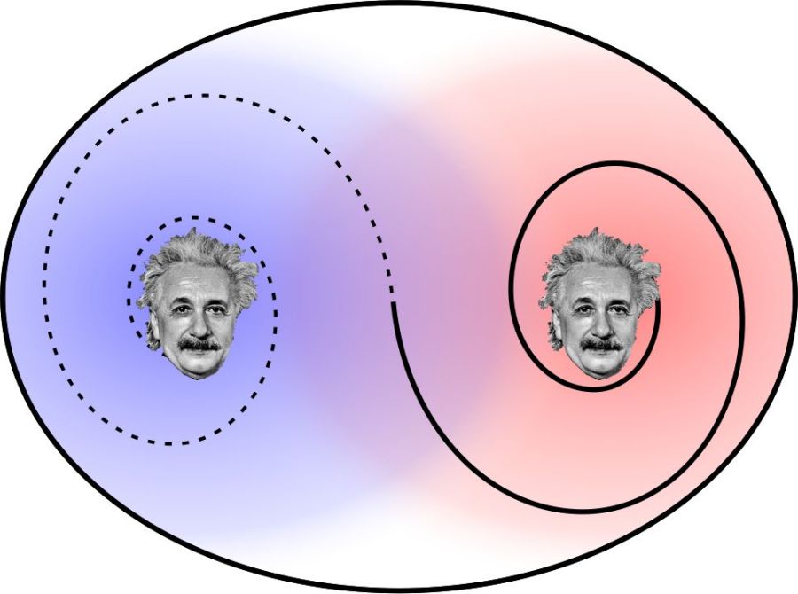
In a sense their supper order arrived in an entangled state.  Our friends knew what was in both boxes together, but they didn’t know what was in either box separately.  Kind of a Schrödinger’s Cat situation — they had to treat each box as 50% baked pasty and 50% fried codfish.

But as soon as Johnny opened one box, he knew what was in the other one even though it was somewhere else.  Jennie could have been in the next room or the next town or the next planet — Johnnie would have known, instantly, which box had his meal no matter how far away that other box was.

By the way, Jennie was free to open her box on the way home but that’d make no difference to Johnnie — the box at his place would have stayed a mystery to him until either he opened it or he talked to her.

Entangled 2Information transfer at infinite speed?  Of course not, because neither hungry person knows what’s in either box until they open one or until they exchange information.  Even Skype operates at light-speed (or slower).

But that’s not quite quantum entanglement, because there’s definite content (meat pie or batter-fried cod) in each box.  In the quantum world, neither box holds something definite until at least one box is opened.  At that point, ambiguity flees from both boxes in an act of global correlation.

There’s strong experimental evidence that entangled particles literally don’t know which way is up until one of them is observed.  The paired particle instantaneously gets that message no matter how far away it is.

Niels Bohr’s Principle of Complementarity is involved here.  He held that because it’s impossible to measure both wave and particle properties at the same time, a quantized entity acts as a wave globally and only becomes local when it stops somewhere.

Here’s how extreme the wave/particle global/local thing can get.  Consider some nebula a million light-years away.  A million years ago an electron wobbled in the nebular cloud, generating a spherical electromagnetic wave that expanded at light-speed throughout the Universe.

cats-eye nebula
The Cat’s Eye Nebula (NGC 6543)
courtesy of NASA’s Hubble Space Telescope

Last night you got a glimpse of the nebula when that lightwave encountered a retinal cell in your eye.  Instantly, all of the wave’s energy, acting as a photon, energized a single electron in your retina.  That particular lightwave ceased to be active elsewhere in your eye or anywhere else on that million-light-year spherical shell.

Surely there was at least one other being, on Earth or somewhere else, that was looking towards the nebula when that wave passed by.  They wouldn’t have seen your photon nor could you have seen any of theirs.  Somehow your wave’s entire spherical shell, all 1012 square lightyears of it, instantaneously “knew” that your eye’s electron had extracted the wave’s energy.

But that directly contradicts a bedrock of Einstein’s Special Theory of Relativity.  His fundamental assumption was that nothing (energy, matter or information) can go faster than the speed of light in vacuum.  STR says it’s impossible for two distant points on that spherical wave to communicate in the way that quantum theory demands they must.

Want some irony?  Back in 1906, Einstein himself “invented” the photon in one of his four “Annus mirabilis” papers.  (The word “photon” didn’t come into use for another decade, but Einstein demonstrated the need for it.)  Building on Planck’s work, Einstein showed that light must be emitted and absorbed as quantized packets of energy.

It must have taken a lot of courage to write that paper, because Maxwell’s wave theory of light had been firmly established for forty years prior and there’s a lot of evidence for it.  Bottom line, though, is that Einstein is responsible for both sides of the wave/particle global/local puzzle that has bedeviled Physics for a century.

~~ Rich Olcott

Think globally, act locally. Electrons do.

“Watcha, Johnnie, you sure ‘at particle’s inna box?”
“O’course ’tis, Jennie!  Why wouldn’t it be?”
“Me Mam sez particles can tunnel outta boxes ’cause they’re waves.”

“Can’t be both, Jessie.”


Double slit experiment
The double-slit experiment.
An electron beam travels from the source at left to a display screen. In between there’s a barrier with two narrow slits.

Maybe it can.

Nobel-winning (1965) physicist Richard Feynman said the double-slit experiment (diagrammed here) embodies the “central mystery” of Quantum Mechanics.

When the bottom slit is covered the display screen shows just what you’d expect — a bright area  opposite the top slit.

When both slits are open, the screen shows a banded pattern you see with waves.  Where a peak in a top-slit wave meets a peak in the bottom-slit wave, the screen shines brightly.  Where a peak meets a trough the two waves cancel and the screen is dark.  Overall there’s a series of stripes.  So electrons are waves, right?

But wait.  If we throttle the beam current way down, the display shows individual speckles where each electron hits.  So the electrons are particles, right?

Now for the spooky part.  If both slits are open to a throttled beam those singleton speckles don’t cluster behind the slits as you’d expect particles to do.  A speckle may appear anywhere on the screen, even in an apparently blocked-off region.  What’s more, when you send out many electrons one-by-one their individual hits cluster exactly where the bright stripes were when the beam was running full-on.

It’s as though each electron becomes a wave that goes through both slits, interferes with itself, and then goes back to being a particle!

By the way, this experiment isn’t a freak observation.  It’s been repeated with the same results many times, not just with electrons but also with light (photons), atoms, and even massive molecules like buckyballs (fullerene spheres that contain 60 carbon atoms).  In each case, the results indicate that the whatevers have a dual character — as a localized particle AND as a wave that reacts to the global environment.

Physicists have been arguing the “Which is it?” question ever since Louis-Victor-Pierre-Raymond, the 7th Duc de Broglie, raised it in his 1924 PhD Thesis (for which he received a Nobel Prize in 1929 — not bad for a beginner).  He showed that any moving “particle” comes along with a “wave” whose peak-to-peak wavelength is inversely proportional to the particle’s mass times its velocity.  The longer the wavelength, the less well you know where the thing is.

I just had to put numbers to de Broglie’s equation.  With Newton in mind, I measured one of the apples in my kitchen.  To scale everything, I assumed each object moved by one of its diameters per second.  (OK, I cheated for the electron — modern physics says it’s just a point, so I used a not-really-valid classical calculation to get something to work with.)

“Particle” Mass, kilograms Diameter, meters Wavelength, meters Wavelength, diameters
Apple 0.2 0.07 7.1×10⁻³³ 1.0×10⁻³¹
Buckyball 1.2×10⁻²⁴ 1.0×10⁻⁹ 0.083 8.3×10+7
Hydrogen atom 1.7×10⁻²⁷ 1.0×10⁻¹⁰ 600 6.0×10+12
Electron 9.1×10⁻³¹ 3.0×10⁻¹⁷ 3.7×10+12 1.2×10+29

That apple has a wave far smaller than any of its hydrogen atoms so I’ll have no trouble grabbing it for a bite.  Anything tinier than a small virus is spread way out unless it’s moving pretty fast, as in a beam apparatus.  For instance, an electron going at 1% of light-speed has a wavelength only a nanometer wide.

Different physicists have taken different positions on the “particle or wave?” question.  Duc de Broglie claimed that both exist — particles are real and they travel where their waves tell them to.  Bohr and Heisenberg went the opposite route, saying that the wave’s not real, it’s only a mathematical device for calculating relative probabilities for measuring this or that value.  Furthermore, the particle doesn’t exist as such until a measurement determines its location or momentum.  Einstein and Schrödinger liked particles.  Feynman and Dirac just threw up their hands and calculated.

Which brings us to the other kind of quantum spookiness — “entanglement.”  In fact, Einstein actually used the word spukhafte (German for “spooky”) in a discussion of the notion.  He really didn’t like it and for good reason — entanglement rudely collides with his own Theory of Relativity.  But that’s another story.

~~ Rich Olcott

Location, Location, Location

“Hoy, Johnny, still got that particle inna box?”
“Sure do, Jessie.”
“So where’s hit in there?”
“Me Pap says hit’s spread-out like but hit’s mostly inna middle.”
“Why’s hit spread then?”
“The more I taps the box, the wider hit spreads. Sommat to do wiff energy.”


PIB0
Newton would have answered Jessie’s question by saying, sort of, “Pick a point anywhere in the box.  The probability that the particle is at that point is equal to the probability that it’s at any other point.” PIB stack

Quantum physicists take a different approach. They start by saying, “We know there’s zero probability that the particle is anywhere outside of the box, so there must be zero probability that it’s exactly at any wall.”

Now for a trick that we’re actually quite used to.  When you listen to an orchestra, you can usually pick out the notes being played by a particular instrument.  Someone blessed/cursed with perfect pitch can tell when a note is just a leetle bit flat, say an A being played at 438 cycles instead of 440. You can create any sound by mixing together the right frequencies in the right proportion. That’s how an MP3 recorder does it.

QM solutions use that strategy the other way round. They calculate probabilities by adding together sets of symmetric elementary shapes, all of which are zero at certain places, like the box walls. For instance, on average Johnnie’s particle will be near the middle of his box, so we start a set with an orange mound of probability right there. That mound is like our base frequency — it has no nodes, no non-wall places where the probability is zero.

Then we add a first overtone, the one-node yellow shape that represents equal probability on either side of a plane of zero probability.

Two nodal planes at right angles give us the four-peaked green shape. Further steps up have more and more nodal planes (cyan then blue, and so on). The video shows the running total up to 46 nodes.

.PIB sum
As we add more nodes, the cumulative shape gets smoother and broader.  After a huge number of steps, the sum will look pretty much like Newton’s (except for right at the walls, of course).

So if the classical and QM boxes wind up looking the same, why go to all that trouble?  Because those nodes don’t come for free.

Inverse tennisSuppose you’re playing goalie in an inverse tennis game.  There’s a player in each service box.  Your job is to run the net line using your rackets to prevent either player from getting a ball into the opposing half-court.  Basically, you want the ball’s locations to look like the single-node yellow shape up above.  You’ll have to work hard to do that.

Now suppose they give you a second, crosswise net (the green shape).  You’re going to have to work twice as hard.  Now add a third net, and so on … each additional nodal plane is going to be harder (cost more energy) to keep empty.  Not a problem if you have an infinite amount of energy.

Enter Planck and Einstein.  They showed there’s a limit for small systems like atoms and molecules.  Electrons dash about in atom- or molecule-shaped boxes, but the principle is the same.  The total probability distribution is still the sum of bounded elementary shapes.  However, you can’t use an infinite number of them.  Rather, you start with the cheapest shapes (the fewest nodes) and build upward.

Tally two electrons for each shape you use.  Why two?  Because that’s the rule, no arguments.

It’s important to realize that QM does NOT say that two specific electrons occupy one shape.  All the charge is spread out over all the shapes — we’re just keeping count.

When you run out of electrons the accumulated model shows everything we can know about the electronic configuration.  You won’t know where any particular electron is, but you’ll know where some electron spends some time.  For a chemist that’s the important thing — the peaks and nodes, the centers of negative and positive charge, are the most likely regions for chemical reactions to happen.

Johnnie’s energetic taps make his particle boldly go where no particle has gone before.

~~ Rich Olcott

Particles and Poetry

“Hoy, Johnny, wotcher got inna box?”
“Hit’s a particle, Jessie.”
“Ooo, lovely for you.  Umm… wot’s a particle then?”
“Me Pap says hit’s sommat you calc’late about wiffout knowin’ wot ’tis.”


Pap’s right.  Newton was a particle guy all the way (he was a strong supporter of the idea that light is composed of particles).  One of his most important insights was that he could simplify gravitational calculations if he replaced an object with an equally massive “particle” located at the object’s center of mass.  Could be a planet, or a moon, or that apple — he could treat each of them as a “particle.”  That worked fine for his purposes, because the distances between his object centers were vastly larger than the object sizes.

Fleas
“Great fleas have little fleas upon their backs to bite ’em / And little fleas have lesser fleas and so on infinitum.” ~~ Augustus De Morgan

It took Roche to work out what happens when the distances get small.  Gravitational forces break the original “particles” into littler particles.  And when two of the little ones approach closely enough they break up, and then those break up…  You get the idea.  Take the process far enough and you get Saturn’s Rings, for instance.

But the analysis can keep going.  Consider one “particle” in Saturn’s A-ring.  It’s probably about 3″ across, made of ice, and contains something like 1024 particles that happen to be molecules of H2O.  Each molecule contains 3 nuclei (2 protons and one oxygen nucleus) and 10 electrons, all 13 of which merit “particle” status if you’re calculating molecules.  They’re all held together by a blizzard of photons carrying the electromagnetic forces between them.  The oxygen nucleus contains 16 nuclear particles, each of which contains 3 quarks.  The quark structures would fly apart except for a host of gluons that pass back and forth transmitting the nuclear strong force.  Hooboy, do we got particles.

“Particle” is a slippery word.  For Newton’s purposes, if an object is small relative to its distance from other objects, that was all he needed to know to treat it as a particle.

One dictionary specifies “a small localized object which has identifiable physical or chemical properties such as volume or mass.”  However, there are theoretical grounds to believe that the classic “particle of light,” the photon, has neither mass nor volume.  Physicists have had long arguments trying to devise a good working definition.  Nobelist (1999) Gerard ‘t Hooft ended one such discussion by saying, “A particle is fundamental when it’s useful to think of it as fundamental.”

It may seem a little strange for a physicist to argue for imprecision.  In fact, ‘t Hooft was arguing for a broad, even poetic but still precise understanding of the word.

Poets use metaphor to help us understand the world.  Part of their art is to pack as much meaning as they can into the minimum number of words.  In the same way, scientists use mathematics to pack observed relationships into a simile called an equation  — a brief bit of math may connect and illuminate many disparate phenomena.

Think of physics as metaphor, with numbers.

Newton’s Law of Gravity works for for galaxies roving through a cluster and for basketball-sized satellites orbiting Earth and for stars circling a black hole (if they don’t get too close).  Maxwell’s Equations, just 30 symbols including parentheses and equal signs, give the speed of light and describe the operation of electric motors.  The particle physicists’ Standard Model makes predictions that match experimental results to more than a dozen decimal places.

Good equations are so successful that Nobelist (1963) Eugene Wigner wrote an influential paper entitled The Unreasonable Effectiveness of Mathematics in the Natural Sciences.

We sometimes get into trouble by confusing metaphor with reality.  Poetic metaphors can be carried too far — Hamlet’s lungs were not in fact filling with water from his “sea of troubles.”

Mathematical models can also be carried too far.  Popular (and practitioner) discussion of quantum mechanics is rife with over-extended metaphors.  QM calculations yield only statistical results — an average position, say, plus or minus so much.  It’s an average, but of what?  The “many worlds” hypothesis is an unnecessarily long jump.  There are simpler, less extravagant ways to account for statistical uncertainty. les Etats Unis

~~ Rich Olcott

Perturbed? You’re not the only one

Dolls
Successive approximations
to a real girl, but still not there

It started with the Babylonians.  The Greeks abhorred the notion.  The Egyptians and Romans couldn’t have gotten along without it. Only 1600 years later did Newton gave final polishing to … The Method of Successive Approximations.

Stay with me, we’ll get to The Chicken soon.

Suppose for some weird reason you wanted to know the square root of 2701.  Any Babylonian could see immediately that 2701 is a bit less than 3600 = 602, so as a first approximation they’d guess ½(60 + (2701/60)) = 52.5.  They’d do the multiplication to check: 52.5×52.5 = 2756.25.

Well, 52.5 is closer than 60 but not close enough.  So they’d plug that number into the same formula to get the next successive approximation: ½(52.5 + 2701/52.5) = 51.97.  Check it: 51.97×51.97 = 2700.88.  That was probably good enough for government work in Babylonia, but if the boss wanted an even better estimate they could go around the loop again.

Scientists and engineers tackle a complex problem piecewise.  Start by looking for a simple problem you know how to solve. Adjust that solution little by little to account for the ways in which the real system differs from the simple case.  Successive Approximation is only one of many adjustment strategies invented over the centuries.

The most widely-used technique is called Perturbation Theory (which has nothing to do with the ways kids find to get on their parents’ nerves).  The strategy is to find some single parameter, maybe a ratio of two masses or the relative strength of a particle-particle interaction.  For a realistic solution, it’s important that the parameter’s value be small compared to other quantities in the problem.

Simplify the original problem by keeping that parameter in the equations but assume that it’s zero.  When you’ve found a solution to that problem, you “perturb” the solution — you see what happens to the model when you allow the parameter to be non-zero.

There’s an old story, famous among physicists and engineers, about an association of farmers who wanted to design an optimum chicken-raising operation.  Maybe with an optimal chicken house they could heat the place with the birds’ own body heat, things like that.  They called in an engineering consultant.  He looked around some running farms, took lots of measurements, and went away to compute.  A couple of weeks later he came back, with slides.  (I told you it’s an old story.)  He started to walk the group though his logic, but he lost them when he opened his pitch with, “Assume a spherical chicken…”

Fat chick bank
Henrietta
Fat Chicken Bank by Becky Zee

Now, he may actually have been on the right track.  It’s a known fact that many biological processes (digestion, metabolism, drug dosage, etc.) depend on an organism’s surface area.  A chicken’s surface area could be key to calculating her heat production.  But chickens (for example, our charming Henrietta) have a complicated shape with a poorly-defined surface area.  The engineer’s approximation strategy must have been to estimate each bird as a sphere with a tweakable perturbation parameter reflecting how spherical they aren’t.

Then, of course, he’d have to apply a second adjustment for feathers, but I digress.

Now here’s the thing.  In quantum mechanics there’s only a half-dozen generic systems with exact solutions qualifying them to be “simple” Perturbation Theory starters.  Johnny’s beloved Particle In A Box (coming next week) is one of them.  The others all depend in similar logic — the particle (there’s always only one of them) is confined to a region which contains places where the particle’s not allowed to be. (There’s one exception: the Free Particle has no boundaries and therefore is evenly smeared across the Universe.)

Virtually all other quantum-based results — multi-electron atoms, molecular structures, Feynman diagrams for sub-atomic physics, string theories, whatever — depend on Perturbation Theory.  (The exceptions are topology and group-theory techniques that generally attempt to produce qualitative rather quantitative predictions.)  They need those tweakable parameters.

In quantum-chemical calculations the perturbation parameters are generally reasonably small or at least controllable.  That’s not true for many of the other areas.  This issue is especially problematic for string theory.  In many of its proposed problem solutions no-one knows whether a first-, second- or higher-level approximation even exists, much less whether it would produce reasonable predictions.

I find that perturbing.

~~ Rich Olcott

Another slice of π, wrapped up in a Black Hole crust

Last week a museum visitor wondered, “What’s the volume of a black hole?”  A question easier asked than answered.

Let’s look at black hole (“BH”) anatomy.  If you’ve seen Interstellar, you saw those wonderful images of “Gargantua,” the enormous BH that plays an essential role in the plot.  (If you haven’t seen the movie, do that.  It is so cool.)

A BH isn’t just a blank spot in the Universe, it’s attractively ornamented by the effects of its gravity on the light passing by:

Gargantua 2c
Gargantua,
adapted from Dr Kip Thorne’s book, The Science of “Interstellar”

Working from the outside inward, the first decoration is a background starfield warped as though the stars beyond had moved over so they could see us past Gargantua.  That’s because of gravitational lensing, the phenomenon first observed by Sir Arthur Eddington and the initial confirmation of Einstein’s Theory of General Relativity.

No star moved, of course.  Each warped star’s light comes to us from an altered angle, its lightwaves bent on passing through the spatial compression Gargantua imposes on its neighborhood.  (“Miles are shorter near a BH” — see Gravitational Waves Are Something Else for a diagrammatic explanation.)

Moving inward we come to the Accretion Disc, a ring of doomed particles destined to fall inward forever unless they’re jostled to smithereens or spat out along one of the BH’s two polar jets (not shown).  The Disc is hot, thanks to all the jostling.  Like any hot object it emits light.

Above and below the Disc we see two arcs that are actually images of the Accretion Disc, sent our way by more gravitational lensing.  Very close to a BH there’s a region where passing light beams are bent so much that their photons go into orbit.  The disc’s a bit further out than that so its lightwaves are only bent 90o over (arc A) and under (arc B) before they come to us.

By the way, those arcs don’t only face in our direction.  Fly 360o around Gargantua’s equator and those arcs will follow you all the way.  It’s as though the BH were embedded in a sphere of lensed Disclight.

Which gets us to the next layer of weirdness.  Astrophysicists believe that most BHs rotate, though maybe not as fast as Gargantua’s edge-of-instability rate.  Einstein’s GR equations predict a phenomenon called frame dragging — rapidly spinning massive objects must tug local space along for the ride.  The deformed region is a shell called the Ergosphere.

Frame dragging is why the two arcs are asymmetrical and don’t match up.  We see space as even more compressed on the right-hand side where Gargantua is spinning away from us.  Because the effect is strongest at the equator, the shell should really be called the Ergospheroid, but what can you do?

Inside the Ergosphere we find the defining characteristic of a BH, its Event Horizon, the innermost bright ring around the central blackness in the diagram.  Barely outside the EH there may or may not be a Firewall, a “seething maelstrom of particles” that some physicists suggest must exist to neutralize the BH Information Paradox.  Last I heard, theoreticians are still fighting that battle.

The EH forms a nearly spherical boundary where gravity becomes so intense that the escape velocity exceeds the speed of light.  No light or matter or information can break out.  At the EH, the geometry of spacetime becomes so twisted that the direction of time is In.  Inside the EH and outside of the movies it’s impossible for us to know what goes on.

Finally, the mathematical models say that at the center of the EH there’s a point, the Singularity, where spacetime’s curvature and gravity’s strength must be Infinite.  As we’ve seen elsewhere, Infinity in a calculation is Nature’s was of saying, “You’ve got it wrong, make a better model.”

So we’re finally down to the volume question.  We could simply measure the EH’s external diameter d and plug that into V=(πd3)/6.  Unfortunately, that forthright approach misses all the spatial twisting and compression — it’s a long way in to the Singularity.  Include those effects and you’ve probably got another Infinity.

Gargantua’s surface area is finite, but its volume may not be.

~~ Rich Olcott

Michelson, Morley and LIGO

Two teams of scientists, 128 years apart.  The first team, two men, got a negative result that shattered a long-standing theory.  The second team, a thousand strong, got a positive result that provided final confirmation of another long-standing theory.  Both teams used instruments based on the same physical phenomenon.  Each team’s innovations created whole new fields of science and technology.

Interferometer 1Their common experimental strategy sounds simple enough — compare two beams of light that had traveled along different paths

Light (preferably nice pure laser light, but Albert Michelson didn’t have a laser when he invented interferometry in 1887) comes in from the source at left and strikes the “beam splitter” — typically, a partially-silvered mirror that reflects half the light and lets the rest through.  One beam goes up the y-arm to a mirror that reflects it back down through the half-silvered mirror to the detector.  The other beam goes on its own round-trip journey in the x-direction.  The detector (Michelson’s eye or a photocell or a fancy-dancy research-quality CCD) registers activity if the waves in the two beams are in step when they hit it.  On the other hand, if the waves cancel then there’s only darkness.

Getting the two waves in step requires careful adjustment of the x- and y-mirrors, because the waves are small.  The yellow sodium light Michelson used has a peak-to-peak wavelength of 589 nanometers.  If he twitched one mirror 0.0003 millimeter away from optimal position the valleys of one wave would cancel the peaks of the other.

So much for principles.  The specifics of each team’s device relate to the theory being tested.  Michelson was confronting the æther theory, the proposition that if light is a wave then there must be some substance, the æther, that vibrates to carry the wave.  We see sunlight and starlight, so  the æther must pervade the transparent Universe.  The Earth must be plowing through the æther as it circles the Sun.  Furthermore, we must move either with or across or against the æther as we and the Earth rotate about its axis.  If we’re moving against the æther then lightwave peaks must appear closer together (shorter wavelengths) than if we’re moving with it.Michelson-Moreley device

Michelson designed his device to test that chain of logic. His optical apparatus was all firmly bolted to a 4′-square block of stone resting on a wooden ring floating on a pool of mercury.  The whole thing could be put into slow rotation to enable comparison of the x– and y-arms at each point of the compass.

Interferometer 3
Suppose the æther theory is correct. Michelson should see lightwaves cancel at some orientations.

According to the æther theory, Michelson and his co-worker Edward Morley should have seen alternating light and dark as he rotated his device.  But that’s not what happened.  Instead, he saw no significant variation in the optical behavior around the full 360o rotation, whether at noon or at 6:00 PM.

Cross off the æther theory.

Michelson’s strategy depended on light waves getting out of step if something happened to the beams as they traveled through the apparatus.  Alternatively, the beams could charge along just fine but something could happen to the apparatus itself.  That’s how the LIGO team rolled.

Interferometer 2
Suppose Einstein’s GR theory is correct. Gravitational wave stretching and compression should change the relative lengths of the two arms.

Einstein’s theory of General Relativity predicts that space itself is squeezed and stretched by mass.  Miles get shorter near a black hole.  Furthermore, if the mass configuration changes, waves of compressive and expansive forces will travel outward at the speed of light.  If such a wave were to encounter a suitable interferometer in the right orientation (near-parallel to one arm, near-perpendicular to the other), that would alter the phase relationship between the two beams.

The trick was in the word “suitable.”  The expected percentage-wise length change was so small that eLIGO needed 4-kilometer arms to see movement a tiny fraction of a proton’s width.  Furthermore, the LIGO designers flipped the classical detection logic.  Instead of looking for a darkened beam, they set the beams to cancel at the detector and looked for even a trace of light.

eLIGO saw the light, and confirmed Einstein’s theory.

~~ Rich Olcott

Gravitational Waves Are Something Else

gravitational-gif.0

If you’re reading this post, you’ve undoubtedly seen at least one diagram like the above — a black hole or a planet or a bowling ball makes a dent in a rubber sheet and that’s supposed to explain Gravity.  But it doesn’t, and neither does this spirally screen-grab from Brian Greene’s presentation on Stephen Colbert’s Late Show:rubber-sheet waves_post

<Blush> I have to admit that the graphic I used a couple of weeks ago is just as bad.

Gravitational waves don’t make things go up and down like ocean waves, and they’re definitely not like that planet on a trampoline — after all, there’s nothing “below” to pull things downward so there can’t be a dent.  And gravitational waves don’t do spirals, much.

soundwave
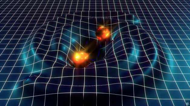
Of all the wave varieties we’re familiar with, gravitational waves are most similar to (NOT identical with!!) sound waves.  A sound wave consists of cycles of compression and expansion like you see in this graphic.  Those dots could be particles in a gas (classic “sound waves”) or in a liquid (sonar) or neighboring atoms in a solid (a xylophone or marimba).

Contrary to rumor, there can be sound in space, sort of.  Any sizable volume of “empty” space contains at least a few atoms and dust particles.  A nova or similar sudden event can sweep particles together and give rise to successive waves that spread as those local collections bang into particles further away.  That kind of activity is invoked in some theories of spiral galaxy structure and the fine details of Saturn’s rings.

In a gravitational wave, space itself is compressed and stretched.  A particle caught in a gravitational wave doesn’t get pushed back and forth.  Instead, it shrinks and expands in place.  If you encounter a gravitational wave, you and all your calibrated measurement gear (yardsticks, digital rangers, that slide rule you’re so proud of) shrink and expand together.  You’d only notice the experience if you happened to be comparing two extremely precise laser rangers set perpendicular to each other (LIGO!).  One would briefly register a slight change compared to the other one.

Light always travels at 186,000 miles per second but in a compressed region of space those miles are shorter.  bent lightEinstein noticed that implication of his Theory of General Relativity and in 1916 predicted that the path of starlight would be bent when it passed close to a heavy object like the Sun.  The graphic shows a wave front passing through a static gravitational structure.  Two points on the front each progress at one graph-paper increment per step.  But the increments don’t match so the front as a whole changes direction.  Sure enough, three years after Einstein’s prediction, Eddington observed just that effect while watching a total solar eclipse in the South Atlantic.

Unlike the Sun’s steady field, a gravitational wave is dynamic. Gravitational waves are generated by changes in a mass configuration.  The wave’s compression and stretching forces spread out through space.

Here’s a simulation of the gravitational forces generated by two black holes orbiting into a collision.  The contours show the net force felt at each point in the region around the pair.
2 black holesWe’re being dynamic here, so the simulation has to include the fact that changes in the mass configuration aren’t felt everywhere instantaneously.  Einstein showed that space transmits gravitational waves at the speed of light, so I used a scaled “speed of light” in the calculation.  You can see how each of the new features expands outward at a steady rate.

Even near the violent end, the massive objects move much more slowly than light speed.  The variation in their nearby field quickly smooths out to an oval and then a circle about the central point, which is why the calculated gravity field generates no spiral like the ones in the pretty pictures.

Oh, and those “gravity well” pictures?  They’re not showing gravitational fields, they’re really gravitational potential energy diagrams, showing how hard it’d be to get away from somewhere.  In the top video, for example, the satellite orbits the planet because it doesn’t have enough kinetic energy to get out of the well.  The more massive the attractor, the tighter it curves space around itself and the deeper the well.

~~ Rich Olcott

Three LIGOs make a Banana Slicer

Ponder for a moment what Space throws at you.  Photons of all sizes, of course —  infra-red ones that warm your skin, visible ones that show you the beach, ultra-violet ones that give you tan and sunburn.  Neutrinos and maybe dark matter particles that pass right through you without even pausing.  All of those act upon you in little bits at little places — gravity pervades you.  You can put up a parasol or step into a cave, but there’s no shielding yourself from gravity.

Gravity’s special character has implications for LIGOs.  A word first about words.  LIGO as a generic noun unwinds to Laser Interferometer Gravitational-Wave Observatory, a class of astronomical instruments. LIGO as a proper noun denotes a project that culminated in the construction of a specific pair of devices that went live in 2002.

That hardware wasn’t sensitive enough to detect the gravitational waves it was created to seek.  To improve the initial LIGO’s power and sensitivity, the LIGO infrastructure and organization morphed into the Advanced LIGO (aLIGO) project.  Concurrently, the LIGO instrument was upgraded and renamed.  No surprise, the instrument’s new name is aLIGO.  An early phase of aLIGO bore uncannily fortunate fruit with the Sept 14 gravitational wave detection.

Four other LIGOs are proposed, under construction or in operation around the world — KARGA in Japan, INDIGO in India, GEO600 in Germany and VIRGO in Italy.  Why so many, and why even consider space-borne LIGOs like LISA Pathfinder and eLISA?

Astronomers ask a series of questions of the Universe:

  • What objects are out there?
  • Where are they?
  • What are they doing?
  • Why are they doing that?

September’s aLIGO incident gave us a gratifyingly unexpected answer to the first question.  To the surprise of theoreticians, the detected event was the collision of two black holes, each of which was in a size range that current theory says shouldn’t be populated.  Even more surprising, such objects are apparently common enough to meet up, form binary pairs and eventually merge.

1 LIGO localizationThe second question is harder.  The best the aLIGO team could do was point to a “banana-shaped region” (their words, not mine) that covers about 1% of the sky.  The team marshaled a world-wide collaboration of observatories to scan that area (a huge search field by astronomical standards), looking for electromagnetic activities concurrent with  the event they’d seen.  Nobody saw any.  That was part of the evidence that this collision involved two black holes.  (If one or both of the objects had been something other than a black hole, the collision would have given off all kinds of photons.)

Why such poor localization?  Blame gravity’s pervasive character and Geometry.  With a telescope, any kind of telescope, you know which direction you’re looking.  Telescopes work only with photons that enter through the front; photons aimed at the back of the instrument stop there.

2 LIGO localization
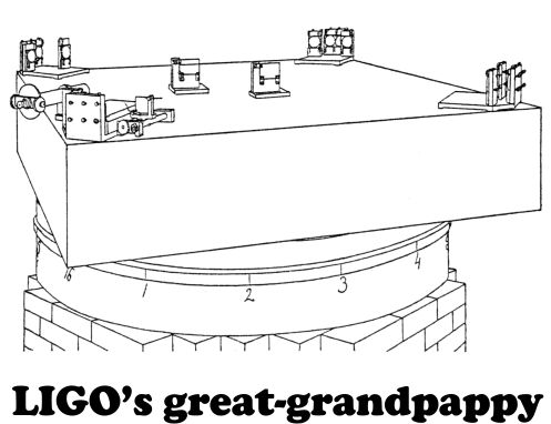
In contrast, a LIGO facility is (roughly speaking) omni-directional.  When a LIGO installation senses a gravitational pulse, it could be coming down from the visible sky or up through the Earth from the other hemisphere — one signal doesn’t carry the “which way?” information.  The diagram above shows that situation.  (The “chevron” is an image of the LIGO in Hanford WA.)  Models based on the signal from that pair of 4-km arms can narrow the source field to a “banana-shaped region,” but there’s still that 180o ambiguity.

The good news is that the LIGO project built not one but two installations, 2500 miles apart.  With two LIGOs (the second diagram) there’s enough information to resolve the ambiguity.  The two also serve as checks on each other — if one sees a signal that doesn’t show up at the other that’s probably a red herring that can be discarded.

3 LIGO localizationThe great “if only” is that the VIRGO installation in Italy was not recording data when the Hanford WA and Livingston LA saw that September signal.  With three recordings to reconcile, the aLIGO+VIRGO combination would have had enough information to slice that banana and localize the event precisely.

When the European Space Agency puts Evolved LISA (eLISA) in orbit (watch the animation, it’s cool) in 2034, there’ll be a million-kilometer triangle of spacecraft up there, slicing bananas all over the sky.

~~ Rich Olcott

The Shape of π and The Universe

pi
This square pi are rounded.

There’s no better way to celebrate 3/14/16 than chatting about how π is a mess but it’s connected to the shape of the Universe, all  while enjoying a nice piece of pie.  I’ll have a slice of that Neil Gaiman Country Apple, please.

The ancient Greeks didn’t quite know what to do about π.  For the Pythagoreans it transgressed a basic tenet of their religious faith — all numbers are supposed to be  integers or at least ratios of integers.  Alas for the faithful, π misbehaves.  The ratio of the circumference of a circle to its diameter just refuses to match the ratio of any pair of integers.

The best Archimedes could do about 250 BCE was determine that π is somewhere between 22/7 (0.04% too high) and 223/71 (0.024% too low).  These days we know of many different ways to calculate π exactly.  It’s just that each of them would take an infinite number of steps to come to a final result.  Nobody’s willing to wait that long, much less ante up the funding for that much computer time.  After all, most engineers are happy with 3.1416.

pi digits
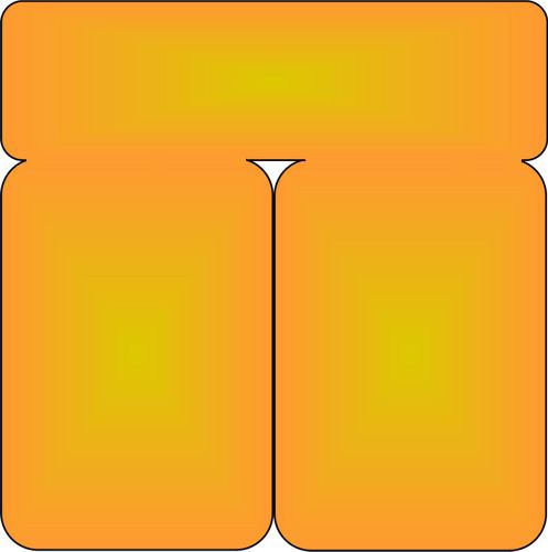
Nonetheless, mathematicians and cryptographers have forged ahead, calculating π to more than a trillion digits.  Here for your enjoyment are the 99 digits that come after digit million….

Why cryptographers ?  No-one has yet been able to prove it, but mathematicians are pretty sure that π’s digits are perfectly random.  If you’re given a starting sequence of decimal digits in π, you’ll be completely unable to predict which of the ten possible digits will be the next one.  Cryptographers love random numbers and they’re in π for the picking.


Another π-problem the Greeks gave us was in Euclid’s Geometry.  Euclid did a great job of demonstrating Geometry as an axiomatic system.  He built his system so well that everyone used it for millennia.  The problem was in his Fifth Postulate.  It claimed that parallel lines never meet, or equivalently, that the angles in every triangle add up to 180o.

Neither “fact” is necessarily true and Euclid knew that — he’d even written a treatise (Phaenomena) that used spherical geometry for astronomical calculations.  On our sweetly spherical Earth, a narwhale can swim a mile straight south from the North Pole, turn left and swim straight east for a mile, then turn left again and swim north a mile to get back to the Pole.  That’s a 90o+90o+90o=270o triangle no problem.  Euclid’s 180o rule works only on a flat plane.

cap areaBack to π.  The Greeks knew that the circumference of a circle (c) divided by its diameter (d) is π.  Furthermore they knew that a circle’s area divided by the square of its radius (r) is also π. Euclid was too smart to try calculating the area of the visible sky in his astronomical work.  He had two reasons — he didn’t know the radius of the horizon, and he didn’t know the height of the sky.  Later geometers worked out the area of such a spherical cap.  I was pleased to learn that π is the ratio of the cap’s area to the square of its chord, s2=r2+h2.

The Greeks never had to worry about that formula while figuring our how many tiles to buy for a circular temple floor.  The Earth’s curvature is so small that h is negligible relative to r.  Plain old πr2 works just fine.

CurvaturesAstrophysicists and cosmologists look at much bigger figures, ones so large that curvature has to be figured in.  There are three possibilities

  • Positive curvature, which you get when there’s more growth at the center than at the edges (balloons and waistlines)
  • Zero curvature, flatness, where things expand at the same rate everywhere
  • Negative curvature, which you get when most of the growth is at the edges (curly-leaf lettuce or a pleated skirt)

Near as the astronomers can measure, the overall curvature of the Universe is at most 10-120.  That positive but miniscule value surprised everyone because on theoretical grounds they’d expected a large positive value.  In 1980 Alan Guth explained the flatness by proposing his Inflationary Universe theory.  Dark energy may well  figure into what’s happening, but that’s another story.

Oh, that was tasty pie.

~~ Rich Olcott